Experiment summary
Overview
This experiment is designed to find out stuff about memory.
Session Types
Each day, each mouse participated in one or more sessions. E.g. in the most common day, a mouse partakes in an open field session, then a virtual reality session, then a second open field session. Our data is organised around these sessions, so it is helpful to understand them to understand the data. The session types are
OF1 and OF2
An open field session. The mouse is placed in a 1m by 1m arena.
VR
A virtual reality session. The mouse is head-fixed, on a wheel in a virtual reality system. The plain VR tag is used for the simplest of our VR tasks, described in … .
VRMC
A virtual reality multi context session. The mouse is head-fixed, on a wheel in a virtual reality system. The reward zone, described above, is in one of two locations in each trail. The mouse is alerted of this change through the walls changing colour.
IMSEQ
Image sequence stuff…
Data
Data overview
Our basic pipeline overview can be found below.
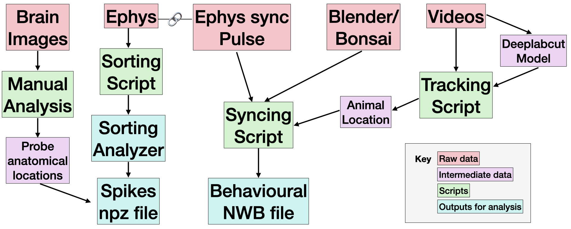
Every session contains an output from Bonsai or Blender, and a Video. These capture the animal behaviour data, as well as a light pulse signal used for synchronisation. Most sessions include ephys data, which capture neural behaviour.
We expect the most useful data to be the outputs for analysis (in teal), or the raw data (in red) or the . Find out how to access the Raw data and Derived data below. We explain how each script was implemented in the Code Protocols section.
Accessing raw data
Folder structure
The raw data is organised as follows:
data_folder/
    session_folder/
        M{mouse}_D{day}_datetime_{session_abbreviation}/
            params.yaml  # metadata about the experiment
            {video_file}.avi  # video of behaviour
            {behaviour_files}.csv  # behavioural output from Bonsai/Blender
            Record Node 102/  # Ephys data
                experiment1/
                    recording1/
                        continous/
                        events/ (not used)
                        spikes/ (not used)
                        structure.oebin
where datetime is the time the session began.
For example, the VR data for mouse 25, day 20 in stored in
"data_folder/vr/M25_D20_2024-11-08_11-52-50_VR1"Find out more about the data below.
Raw Ephys recordings
Stored at
data_folder/Cohort_folder/session_folder/M1_D1_datetime_{session}/Openphys files. Roughly a large binary file with some metadata.
These can be read using spikeinterface e.g.
import spikeinterface.full as si
path_to_recording = "data_folder/of/M25_D20_2024-11-08_11-25-37_OF1/"
recording = si.read_openephys(path_to_recording)
Video files
Stored at
data_folder/Cohort_folder/session_folder/M1_D1_datetime_{session}/{video_name}.aviVideos are named using the BIDS structure, meaning they are of the form sub-{mouse}_day-{day}_ses-{session}_video.avi, e.g. sub-20_day-25_ses-OF1_video.avi.
Open Field gives a top-down view of the open field arena. Used to determine mouse position. Frame rate is 15 frames per second.
VR gives side view of mouse while running. Used to determine Tongue position and pupil dilation. Frame rate is 30 frames per second.
Accessing Derived data
Most of the derived data is in NOLANLABDATASTORE/ActiveProjects/Wolf/COHORT12/. The Sorting Analyzer are kept in NOLANLABDATASTORE/ActiveProjects/Chris/Cohort12/derivatives.
All of this data is synchronized.
Folder structure
Each mouse day (usually) corresponds to one “experiment”, which might contain several “sessions”. To reflect this, the derived data is organised as follows:
derivatives_folder/
    M{mouse}/
        D{day}/
            full/
            {session_type_1}/
            {session_type_2}/
            ...
The information in full is shared between all sessions in the experiment (e.g. if all the data is sorted together, the sorted data is stored here) while information unique to each session is stored in the session_type_n folder. This folder can contain many pieces of data. The data is described below.
Spike data
Stored at
/ActiveProjects/Wolf/COHORT12/M{mouse}/D{day}/{session}/sub-{mouse}_day-{day}_ses-{session}_srt-{sorter_protocol}_clusters.npzContains sorted (but non-curated) clusters. Most importantly each cluster contains a spike train, giving timepoints for each spike in that cluster in seconds. The file is an npz file which can be read using numpy. However, we recommend using pyanpple to open them. The following code snippets loads a file and bins its spike train:
from pathlib import Path
import pynapple as nap

mouse = 25
day = 25
session = "OF1"
srt = "kilosort4"

path_to_active_project = Path("/Volumes/cmvm/sbms/groups/CDBS_SIDB_storage/NolanLab/ActiveProjects/")
session_folder = path_to_active_project / f"Wolf/COHORT12/M{mouse}/D{day}/{session}/"
clusters_file = session_folder / f"sub-{mouse}_day-{day}_ses-{session}_srt-{srt}_clusters.npz"

clusters = nap.load_file(clusters_file)

# print the time stamps of cluster 19
print(clusters[19])
We also store metadata. All the metadata can be accessed through clusters.metadata. This includes:
Quality metrics of each cluster, taken from the SortingAnalyzer, which can be used to curate:
# Find all clusters with a firing rate greater than 10, then subselect using these
high_firing_clusters = clusters[clusters['firing_rate'] > 10]

# Print how many clusters there are with a high firing rate
print(len(high_firing_clusters))
Anatomical information for each cluster. This is the estimate position of the cluster in the brain. We can access the stereotaxic coordinds, common coordinate framework or the estimated brain region as follows:
# print the brain region of cluster 6:
clusters['brain_region'][6]

# print the CCF coords of cluster 12:
CCFs = clusters[['coord_CCFs_z', 'coord_CCFs_y', 'coord_CCFs_x']]
print(CCFs.iloc[12])

# print the SC coords of cluster 16:
SCs = clusters[['coord_SCs_x','coord_SCs_y','coord_SCs_z']]
print(SCs.iloc[16])
Behavioural Data
Stored at
/ActiveProjects/Wolf/COHORT12/M{mouse}/D{day}/{session}/sub-{mouse}_day-{day}_ses-{session}_srt-{sorter_protocol}_beh.nwbThese are NeurodataWithoutBorder files. Can be read with the pynwb or matnwb packages, but we recommend using pynapple. The behavioural data stored depends on the session
Regardless of session type, they are loaded the same way, and we can investigate what is saved in them as follow:
from pathlib import Path
import pynapple as nap

mouse = 25
day = 25
session = "OF1"

path_to_active_project = Path("/Volumes/cmvm/sbms/groups/CDBS_SIDB_storage/NolanLab/ActiveProjects/")
session_folder = path_to_active_project / f"Wolf/COHORT12/M{mouse}/D{day}/{session}/"
beh_file = session_folder / f"sub-{mouse}_day-{day}_ses-{session}_beh.nwb"

beh = nap.load_file(beh_file)

# see what is saved
print(beh)
We’ll discuss the most important data that we save below:
OF behavioural data
- P_x and P_y. Time series of position in cartesian coordinates, in units of cm.
- S. Time series of computed speed of mouse, in cm/s.
- moving. Interval set of whether or not the mouse is moving, with threshold ?? (WOLF).
VR behavioural data
- P. Time series of position along the VR track, in units of cm.
- S. Time series of computed speed along the VR track, in units of cm.
- moving. Interval set of whether of not the mouse is moving.
- lick. Time series of when the mouse licks.
- eye_dilation. Time series of pupil dilation, in dimensionless units.
- trials. Interval set of trails. Used to pick out individual trails.
- trial_type. Time series of which trial type is active at any time point. Type 0 is uncued and type 1 is cued.
Example code
We use pynapple to combine behavioral and spiking data. For example, to compute the most basic positional turning curve in VR we can run
beh = nap.load_file(beh_file)
clusters = nap.load_file(clusters_file)

positional_tuning_curves = nap.compute_1d_tuning_curves(
    group=clusters,
    feature=beh['P'],
    nb_bins=50,
)
which we can plot…
import matplotlib.pyplot as plt

cluster_id = 4

fig, ax = plt.subplots()
ax.plot(positional_tuning_curves[cluster_id])
ax.set_xlabel("Position along track")
ax.set_ylabel("Firing rate (Hz)")
fig.savefig("positional_tuning_curve_cluster_{cluster_id}.pdf")
The real power of pynapple is dealing with time sub-selection using the epoch concept (read more).
In the following code we compute a 1D tuning curve only when the mouse is moving and only during cued trails:
beaconed_trials = beh['trials'][beh['trials']['type'] == 'b']
moving_and_beaconed = beh['moving'].intersect(beaconed_trials)

positional_tuning_curves = nap.compute_1d_tuning_curves(
    group=clusters,
    feature=beh['P'],
    nb_bins=50,
    ep=moving_and_beaconed,
)
SortingAnalyzer
Stored at
/ActiveProjects/Chris/Cohort12/derivativesA spikeinterface SortingAnalyzer object, containing spike times and dervied information such as unit templates, spike locations etc. The analyzer depends on the sorter used. We label each sorting protocol by a number. The details of the protocols can be found in the Protocols section.
Can be read using spikeinterface
import spikeinterface.full as si
sa_path = "derivatives/M25/D20/full/kilosort4/kilosort4_sa"
sorting_analyzer = si.read_sorting_analyzer(sa_path)
Used for more intricate curation and for comparisons of different spike sorters. Our default sorting is the protocol kilosort4.
Read more about SortingAnalyzers here, here and here (video).
Technical details
Code Protocols
Hello!
Experimental Protocols
add links to nolanlab wiki for surgery protocol for neuropixel implantation add links to nolanlab wiki for experimental protocol including behaviour, water dep etc add links to nolanlab wiki for extracting coordniates from DiI tracks using Probe-TRACK and custom scripts add links to nolanlab wiki for extracting features from video including licks, pupil dilation, steps and pose anything else?
Feature Extraction from video data
How do we extract behavioural variables from video footage? Deeplabcut! We manually labelled the pixel location for features of interest from raw video data. We then trained bespoke deeplabcut models to infer pixel positions for each video in the dataset.
Open field videos captured the mouse’s movement in the square arena with a birds eye view. We estimated the mouse’s pose using five features including head, shoulders, middle, tail start and tail end. Pixel coordinates coordinates were transformed and scaled to match the 1 m x 1 m dimensions of the open arena. To estimate head direction, we took the vector between the head and middle features and calculated an angle relative to north.
Add image or gif?
Virtual reality videos captured a side view of the mouse while head-restraint on a cylindrical treadmill. We estimated the mouse’s pupil diameter using eight features including eye north, eye north-east, eye-east etc. Pupil diamter was defined as the average pixel distance between opposite features such as north vs south, north-east vs south-west etc. Units for pupil diameter are arbitrarily defined as we were only concerned with relative changes.
add image or gif of pupil models
We estimated when the mouse’s was engaged in licking using a single feature marking the position of the tongue. When the tongue was out of sight (in the mouse’s mouth), we marked the tongue’s position as the bottom of the mouth. Plotting the tongues position across a session typically produced a point cloud with two clearly defined clusters. To label positions attributable to lick events, we manually drew around the lower positioned cluster. Finally we visually verified this method by creating gif snippets for each session and accessing whether licks were labelled accurately.
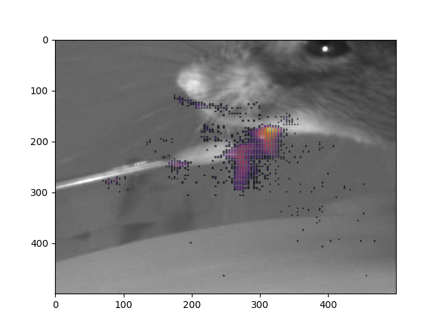
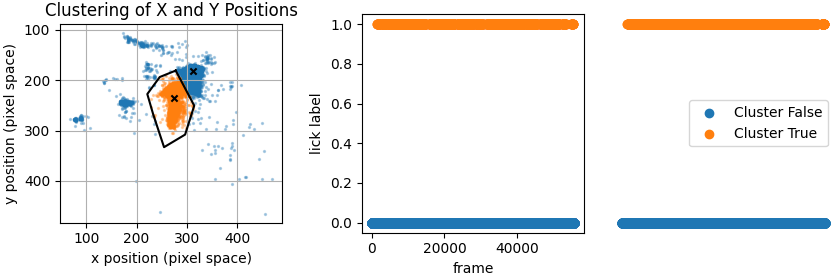
add image or gif of lick models
Experimental details
We stereotaxically targeted the medial entorhinal cortex of 7 males and 1 female C57BL/6J mice with Neuropixel 2.0 (NP2; 4 shank) probes. Prior to implantation of the NP2 probes, mice were trained in the VR linear track experiment to an expert level in both beaconed and non-beaconed trial variants (see Tennant et al., 2018; 10.1016/j.celrep.2018.01.005).
Changes to the task from Tennant et al., 2018, Tennant et al., 2022 and Clark and Nolan, 2024 (T18, T22 and C24 respectively):
- Water deprivation was used instead of food deprivation therefore 10% sucrose solution was used as reward instead of soy milk. The volume of sucrose solution varied between 5-10 uL per reward dispensed.
- A speed of 3 cm/s was used as the stop threshold, compared to 0.7 cm/s and 4.7 cm/s used in T18 and T22.
- Probe trials (non-beaconed trials without reward) were not recorded in this experiment.
- Upon teleportation back to the start of the track, trial type was randomised with equal weighting to beaconed and non-beaconed trials, this produced an equal number of beaconed and non-beaconed trials compared to the repeated block structures used in T18 and T22.
- Mice were only implanted once they reached an expert level in the task.
- Electrophysiology was acquired using a National Instruments/IMEC acquisition system and recorded using Open Ephys software using the Neuropixel acquisition external plugin.
- Behavioural variables were stored and saved directly from Blender3D, and time synced retrospectively using aperiodic TTL pulses sent directly to both the Neuropixel acquisition system and Blender3D via a custom Arduino Due.
FAQ
How was the experiment conducted on a typical day?
Experimental days involved recording from mice in the open arena and then in the virtual location memory task and then once again in the open arena. Mice were collected from the holding room 30 - 60 minutes before recording, were handled for 5 - 10 minutes, weighed and placed for 10 - 20 minutes in a cage containing objects and a running wheel. Between recording sessions mice were placed back in the object-filled playground for 10 - 20 minutes. The open arena consisted of a metal box with a square floor area, removable metal walls, metal frame (Frame parts from Kanya UK, C01-1, C20-10, A33-12, B49-75, B48-75, A39-31, ALU3), and an A4-sized cue card in the middle of one of the metal walls. For the open field exploration session, mice were placed in the open arena while tethered via an ultrathin Neuropixel aquisition cable No Commutator was used. In a small number of sessions, tangling of the Neuropixel cable caused the cable to fall in front of the mouse. To stop mice from knawing on the cable, Mice were quickly untangled by the experimentor. For the location memory task water-restricted mice were trained to obtain rewards at a location on the virtual linear track. Mice were head-fixed using a RIVETS clamp (Ronal Tool Company, Inc) and ran on a cylindrical treadmill fitted with a rotary encoder (Pewatron). Virtual tracks, generated using Blender3D (blender.com) had length 200 cm, with a 60 cm track zone, a 20 cm reward zone, a second 60 cm track zone and a 60 cm black box to separate successive trials. The distance visible ahead of the mouse was 50 cm. The reward zone was either marked by distinct vertical green and black bars on beaconed trials, or was not marked by a visual cue at all on non-beaconed. A feeding tube placed in front of the animal dispensed 10 % sucrose water rewards (5 - 10 5l per reward) if the mouse stopped in the reward zone. A stop was registered in Blender3D if the speed of the mouse dropped below 3 cm/s. Speed was calculated on a rolling basis from the previous 100 ms at a rate of 60 Hz. Trials were delivered in a random fashion with a equal probability on any given trial of being beaconed or non-beaconed. Mice were trained to an expert level in the location memory task before being implanted with Neuropixel 2.0 probes and undergoing the three session (open arena/location memory task/open arena) For more details, see Clark and Nolan 2024, https://doi.org/10.7554/eLife.89356.2
How was data collected?
Electrophysiological signals were acquired using a Neuropixel 2.0 headstage connected via an Neuropixel aquisition cable attached to an IMEC-National Instruments aquisition system (recommended hardware as of July 2024). For the location memory task, positional and trial information was saved in Blender3D at 60 Hz and time sync with TTL pulses delivered concurrently to the Neuropixel aquisition system and the Blender3D computer via an arduino Due. In the open arena, motion and head-direction tracking used a camera (Logitech B525, 1280 x 720 pixels Webcam, RS components 795-0876) attached to the celing of the frame. A custom bonsai tracking script picked up the TTL pulses delivered to an LED in sight of the tracking camera and out of sight of the freely exploring mouse. Body and head direction tracking was completed post-recording using DeepLabCut.
What was the surgery schedule of the experiment?
Mice underwent two seperate surgeries under anaesthesia, the first being a headpost attachment surgery followed by a Neuropixel 2.0 implantation mounted on a Apollo drive resuable 3D printed body. All surgeries were performed by Harry Clark
What drugs were used in the experiment?
Isoflurane used during surgery. Vetergesic jelly given post surgery. Carprofen and Buprenorphine were given subcutaneously at the recommended dosage post surgery
How can I reproduce the stereotaxic surgery?
Add this
Where can I find files for 3D printing the reusable 3D printed components?
Add this Include rivets custom designs
Where can I find the used NP2 probes for use in future experiments?
There are currently 4 x NP2 4-shank probes ready to be used for implantation. These can be found within the 2nd floor wet lab room (add room number) in the drive building area. A box labelled with “Neuropixel 2.0 4 shank probes, Harry Clark” can be found on the shelf above the drive building bench in the drive staging area (marked by yellow tape). (This information was accurate as of 04/03/2025). These drives are super-glued to an Apollo drive shuttle and thus can only be used for further experimentation with Apollo drive compatible components.
Still missing a vital piece of information?
Email harrydclark91@gmail.com for further clarification so we can add the relevant information to this document.
References
Tennant et al., 2018; 10.1016/j.celrep.2018.01.005 Tennant et al., 2022; 10.1016/j.cub.2022.08.050 Clark and Nolan, 2024; 10.7554/eLife.89356.3